Week 03
Basics of Neural Networks (Part 2)

LLMs in Lingustic Research WiSe 2024/25

Akhilesh Kakolu Ramarao

HHU

23 Oct 2024

Activation functions

Activation functions are used to introduce non-linearity to the output of a neuron.

Sigmoid function \[ f(x) = \frac{1}{1 + e^{-x}} \]

Example: \(f(0) = 0.5\)

where:

- f(x): This represents the output of the sigmoid function for a given input x.
- e: This is the euler's number (approximately 2.71828).
- x: This is the input to the sigmoid function.
- 1: This is added to the denominator to avoid division by zero.

The sigmoid function takes any real number as input and outputs a value between 0 and 1.
It is used in the output layer of a binary classification problem.

ReLU function

\[ f(x) = \max(0, x) \]

Example: \(f(2) = 2\)

where:

- f(x): This represents the output of the ReLU function for a given input x.
- x: This is the input to the ReLU function.
- max: This function returns the maximum of the two values.
- 0: This is the threshold value.

The Rectified Linear Unit (ReLU) function is that outputs the input directly if it is positive, otherwise, it outputs zero.
The output of the ReLU function is between 0 and infinity.
It is a popular activation function used in deep learning models.

Loss functions

During forward pass, the neural network makes predictions based on input data.
The loss function compares these predictions to the true values and calculates a loss score.
The loss score is a measure of how well the network is performing.
The goal of training is to minimize the loss function.
You can use different loss functions for different set of tasks:
- For regression problems, use MSE or MAE.
- For classification problems, use cross-entropy loss.
- For multi-class classification problems, use categorical cross-entropy loss.

Gradient descent

Gradient descent is a optimization algorithm used in machine learning to minimize the loss function of a model.
The algorithm works by iteratively adjusting the model parameters (weights and biases) to reduce the loss.
The key idea behind gradient descent is to move in the direction of the negative gradient of the loss function.
A negative gradient indicates the direction of steepest descent, i.e., the direction in which the loss decreases the fastest.
By following the gradient, the algorithm can find the optimal values of the model parameters that minimize the loss function.

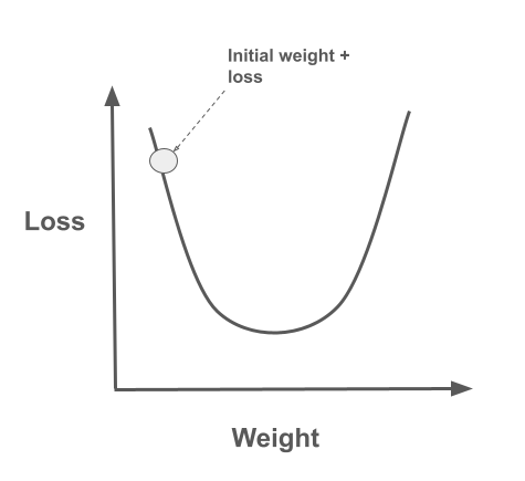
X-axis (Weight): Represents the value of the model parameter being optimized.
Y-axis (Loss): Represents the value of the loss function being minimized.
The goal is to find the value of the model parameter that minimizes the loss function.

The process starts at an initial weight with a corresponding loss, marked as “Initial weight + loss” on the graph
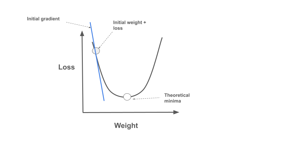
Gradient: The algorithm calculates the gradient (slope) at the current position. This gradient indicates the direction of steepest ascent.

The model then takes a step in the opposite direction of the gradient, as we want to minimize the loss.
This is why it’s called gradient descent - we descend along the gradient.
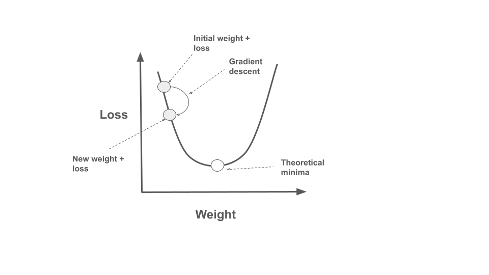
The “New weight + loss” point on the graph shows an intermediate step in this process, where the loss has decreased compared to the initial position.

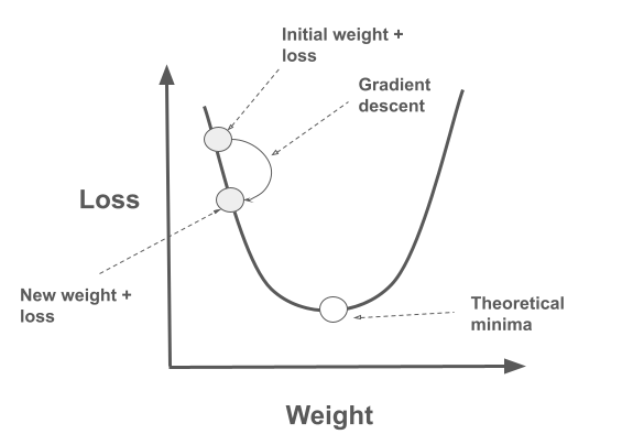
As the algorithm progresses, it should ideally approach the bottom of the curve, labeled as “Theoretical minima” in the image.
The algorithm may not always reach the exact theoretical minima due to factors like step size (learning rate) and the complexity of the loss landscape.
But, it typically converges to a point close enough to be practically useful for model optimization.

Learning rate

The learning rate is a hyperparameter that controls how much the model parameters are adjusted during training.
A hyperparameter is a parameter whose value is set before the learning process begins.
Learning rate is a critical parameter that can affect the convergence of the optimization algorithm.
A high learning rate can cause the model to overshoot the minima, leading to instability and divergence.
A low learning rate can slow down the training process and may get stuck in local minima.

Single-layer Neural Network

A neural network is a collection of interconnected nodes (neurons) that process input data to produce output predictions.
The nodes are organized into layers, with each layer performing specific computations.
The input layer receives the input data, the hidden layers process the data, and the output layer produces the final predictions.
The connections between nodes are represented by weights, which are adjusted during training to optimize the model.

flowchart LR
    %% Input Layer
    I1((I1)):::inputStyle
    I2((I2)):::inputStyle
    I3((I3)):::inputStyle
    B1((Bias)):::biasStyle
    %% Hidden Layer
    H1((H1)):::hiddenStyle
    H2((H2)):::hiddenStyle
    H3((H3)):::hiddenStyle
    B2((Bias)):::biasStyle
    %% Output Layer
    O1((O1)):::outputStyle
    O2((O2)):::outputStyle
    %% Connections
    I1 -->|w11| H1
    I1 -->|w12| H2
    I1 -->|w13| H3
    I2 -->|w21| H1
    I2 -->|w22| H2
    I2 -->|w23| H3
    I3 -->|w31| H1
    I3 -->|w32| H2
    I3 -->|w33| H3
    B1 -->|b1| H1
    B1 -->|b2| H2
    B1 -->|b3| H3
    H1 -->|v11| O1
    H1 -->|v12| O2
    H2 -->|v21| O1
    H2 -->|v22| O2
    H3 -->|v31| O1
    H3 -->|v32| O2
    B2 -->|b4| O1
    B2 -->|b5| O2
    %% Styles
    classDef inputStyle fill:#3498db,stroke:#333,stroke-width:2px;
    classDef hiddenStyle fill:#e74c3c,stroke:#333,stroke-width:2px;
    classDef outputStyle fill:#2ecc71,stroke:#333,stroke-width:2px;
    classDef biasStyle fill:#f39c12,stroke:#333,stroke-width:2px;
    %% Layer Labels
    I2 -.- InputLabel[Input Layer]
    H2 -.- HiddenLabel[Hidden Layer]
    O1 -.- OutputLabel[Output Layer]
    style InputLabel fill:none,stroke:none
    style HiddenLabel fill:none,stroke:none
    style OutputLabel fill:none,stroke:none

The input layer consists of three nodes (I1, I2, I3) representing the input features.
The hidden layer consists of three nodes (H1, H2, H3) that process the input data.
The output layer consists of two nodes (O1, O2) that produce the final predictions.
The connections between nodes are represented by weights (w11, w12, …, v32) and biases (b1, b2, …, b5).
The weights and biases are adjusted during training to optimize the model.
The model makes predictions by passing the input data through the network and computing the output.

Training, development and test datasets

The training dataset is used to optimize the model parameters (weights and biases) using gradient descent.
The development dataset is used to tune the hyperparameters of the model, such as the learning rate and the number of hidden units.
The test dataset is used to evaluate the performance of the model on unseen data.
In order to avoid overfitting, it is important to have separate datasets for training, development, and testing.
The training dataset is typically the largest, followed by the development and test datasets.
The development and test datasets should be representative of the data the model will encounter in the real world.
The datasets should be randomly sampled to avoid bias and ensure that the model generalizes well.

Week 03 Basics of Neural Networks (Part 2)